Statistics: the most important tool, and the most abused
Reliable statistics inform individual predictions without settling how people may be treated. Evidence, treatment, and publication require distinct judgments.
Builds on the Assumptions and Essay 01: there is a way things are, and a claim says something to the extent it changes what we should expect.1
Here’s a fact about the world: Distributions are how you see a society. They tell you how something is spread across a population: how common it is, how often it occurs, and how much people differ. There is a parallel to a gas here. Describing a gas particle by particle is hopeless; there are far too many of them. The gas gets described anyway, as a whole, and the description never names a single molecule. People are society’s particles.
And so it follows that a distribution is not a verdict on the person in front of you. What is true of a group does not automatically tell you what is true of any particular member of it. The second claim does not cancel the first, and the first does not license ignoring the second. A still picture of an ordered society or culture is an average of people moving in every possible direction.
Many public arguments about groups are really fights between two mistakes. One side holds that the first claim implies a verdict. The other holds that the second claim makes the group-level description useless, or close to harmful. The first camp cites the numbers and worries that the other cannot count. The second distrusts the inference and worries that the first is bigoted. Each worry is sometimes justified.
These are different errors. Ignoring good evidence is one; turning a group-level pattern into a judgment about an individual is another. We need to avoid both. And even a correct distribution does not, by itself, tell us how anyone should be treated or how the finding should be communicated. Those require further arguments.
1. You have never seen a society
You have never seen a society. Neither have I. What each of us has seen is, at most, a few thousand people, filtered by where we live, what we do, and what gets shown to us — a sample so skewed that no honest method would accept it. Yet questions about societies are real questions with real answers: is this disease spreading; are wages rising; is crime falling; do children from this district end up poorer than children from that one. For questions of how many and how often, there is no substitute for counting. Whoever answers them is using an aggregate. The only choice is between measured aggregates and imagined ones — between counting, and generalising your news feed.
The gas parallel is worth a moment, because it shows what counting buys. A litre of air, the space inside a milk carton, holds about twenty-five thousand billion billion molecules, a 25 followed by twenty-one zeros.2 No one has followed one of them, and no one needs to. In 1860 James Clerk Maxwell described how fast the molecules of a gas move without tracking a single molecule: he gave the law by which their speeds are spread, and from it how many move within any range of speeds.3 The particles are out of reach. The gas is not. A distribution is not a poor substitute for seeing every particle; at that scale, it is the description.
When someone puts a finding about a group on the table, honest answers include these three: it’s wrong, and here is a better measurement; it’s right, and here is what it actually means; it’s unreliable, and here is the flaw in how it was made. Each of those answers the evidence.
“You cannot say that about a group” answers something else, and it is worth asking what. Sometimes it means that isn’t true, with no evidence offered. Sometimes it means that may be true, but saying it this way, to this audience, will do harm. The second needs an argument about publishing, not about truth, and it is a fair thing to argue about.
So I keep two questions apart: is it true, and should I publish it, and how? Foreseeable harm can be a reason not to publish, or to publish more carefully. It is no reason to think the finding false. Political discomfort doesn’t settle the second question, and neither does a bare “someone might misuse it”. My default is to publish. Not because publishing is always harmless, but because I don’t trust anyone, myself included, to judge reliably when silence is better. So if I want to hold a finding back, the burden is on me to make the case, and where I can, to have someone else check it. Holding back has costs too: decisions get worse, harms stay hidden, and nobody can check the finding. Calling something a publication risk settles neither its truth nor what should be done about it. And none of this gives me any automatic right to stop someone else publishing.4
A distribution is knowledge. It is often the only knowledge available at the scale of millions. A society that will not look at its own distributions is flying blind by choice: the instruments are there, and it has unplugged them.
2. Particles answer; people don’t, and some lie
Counting people is harder than counting molecules, and not only because there are fewer of them. Every molecule in Maxwell’s gas takes part in the distribution; none sits it out, and none pretends to a speed it does not have. People differ from particles in two ways, and I want to keep them apart, because they are different problems with different remedies.
First, people do not all answer. In 1936 the Literary Digest mailed about ten million ballots asking who would win the presidency. Nearly 2.4 million came back, roughly one in four. The magazine called it for Landon, 54 to 41. Roosevelt won with 61 percent.5 The diagnosis has been argued over ever since: who was sent a ballot, and who sent it back. Either way the trouble was who answered, not what they said. That problem has grown, not shrunk. A typical telephone survey in the United States got an answer from 36 percent of the people it called in 1997. By 2018 it got one from 6.6 A low rate does not by itself make a poll wrong; the people who publish those rates say so. It means the few who answered have to stand in for the many who did not. When polls miss, this is where the inquiries look. British polls in 2015 called a tie; the Conservatives won by seven points, and the inquiry named unrepresentative samples as the primary cause and rejected deliberate misreporting. American polls in 2016 were off by about two points nationally and about five at state level, and the review found no evidence that voters had hidden their support for Trump.7 A particle never declines to be counted. People decline all the time, and the ones who decline differ from the ones who don’t.
Second, people who do answer sometimes lie, and the lies run in a known direction. After the 2008 American election, 78 percent of respondents to a major academic election survey said they had voted. About 57 percent of those eligible had.8 Twenty-one points separate what people said from what the count says, and the non-voters most likely to claim a vote were the politically engaged ones. Ask about abortion and the shading runs the other way: fewer than half the abortions performed in the United States over one five-year span were reported by the women who had them.9 On sensitive topics misreporting is common, and which way people shade depends on what the question makes them look like.
Two further troubles follow, and neither has a parallel in the gas. The wording of the question changes the answer. In 1974 a national American survey asked whether most men are better suited emotionally for politics than most women. Offered agree or disagree, 47 percent agreed. Offered a balanced pair of statements to choose between, 33 percent did.10 Fourteen points moved because the sentence changed shape, not because the people did. And the records lie too, so “check the record instead” is not a clean escape. The 2020 United States census was checked afterwards against an independent survey. It had missed about one Black resident in thirty and one Hispanic resident in twenty, and counted white residents about one and a half in a hundred too many. The national total was off by a quarter of one percent, because the misses and the double counts largely cancelled.11 A record is somebody’s count, made by somebody’s method. Arrest data, which I come to below, measure policing as well as crime.
None of this is a reason to stop counting people. It is a reason to ask, of every number about a society, who was asked, who answered, what exactly they were asked, and what they had reason to say. Those questions have answers, and a careful study gives them. The point is narrower: the third honest response above, it’s unreliable, and here is the flaw in how it was made, is far more often the right one for a poll than for a pressure gauge. A gas cannot refuse the question and cannot shade its answer. A society can do both, and does.
3. What a distribution actually says
Now I want to look closely at what a distribution is knowledge of. The opposite abuse, turning a number into a verdict on a person, begins exactly where this goes unexamined.
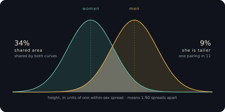
Take the most boring true group difference in the world: men are taller than women. The gap is real, large by the standards of social science, and visible wherever height has been measured. Measured is the word. These heights were taken with an instrument, not asked for, and nobody can shade a reading. Most facts about a society are not like that; they come from asking. Now watch what the sentence compresses away. Pick a man and a woman at random from the adult population of a country like the United States, and in about one pairing in eleven, she is the taller one.12 Not a rounding error — one in eleven. The two distributions are distinct, and they overlap substantially: about a third of the area under one curve sits under the other. (That is a different number from the one in eleven, measuring something else; the figure below shows both.) “Men are taller than women” is a true sentence about two curves. It lets you make a good guess about a pair picked at random; it cannot promise which of the next two people through the door is taller.
Second lesson, from the strongest statistical claim in public health. Smoking causes lung cancer: the evidence is about as close to certainty as observational science gets, and the risk multiplier is enormous — on the order of twentyfold. And most smokers never get lung cancer.13 Both facts, at full strength. Which is why your uncle who smoked to ninety proves nothing: the claim was never “every smoker dies of it”. And it is why a doctor who told one particular smoker “you will get cancer” would be claiming far more than the evidence supports. The causal claim is about the whole population: it says what happens to rates when a population smokes. The abuse of the anecdote against the aggregate (“my uncle…”) and the abuse of the aggregate against the person (“you will…”) are the same arithmetic error, committed in opposite directions.
So a reliable, relevant group number can tell you something about the person in front of you. How much depends on how well it fits their case and on what else you know about them. Learning more about them does not automatically cancel it. But it gives odds, not certainty, and odds alone never settle how you may treat someone.14 Measuring someone’s height can settle a question the average only helped you guess. Learning something about them that has nothing to do with height does not. What counts is what new information tells you about the question, not merely that it is about this particular person.
4. The arithmetic of the accusation
The error becomes vicious in one specific case: when the trait in question is rare and bad.
Here is a fact I owe you in passing, because the essays that follow will need it. In the most recent global count, about nine in ten of the people brought into contact with the police as suspects in intentional homicide were men.15 That is a count of suspects, in the countries that report them, in one year, not of every killer everywhere. But it is no one-year accident: earlier editions of the same study report the same lopsided share. And it is larger than almost any group difference the loudest debates are about. Now do the arithmetic that the accusation skips. Killing is mercifully rare. Take a difference that large in a trait that rare, and ask: given this man in front of me, what did the statistic tell me about him? The probability that a randomly chosen man was recorded for a homicide this year is minuscule; the probability for a woman, roughly nine times smaller. Nine to one compares two tiny numbers. It does not make either of them big.
A statistician will rightly press one point, and it answers a different question. Once a homicide has happened, the nine-in-ten share is the relevant number for the question “who did it?”. Among otherwise unknown suspects, being a man multiplies the odds about ninefold. That is exactly where profiling begins, and the arithmetic does not forbid it. What keeps it from becoming a verdict is the rest of the reasoning. The probability for any one man stays small until other evidence narrows the field. And what anyone may do with that probability (stop, search, suspect) needs its own justification.
Three different quantities, one word "nine to one"
An illustrative population, not a homicide estimate. Two groups of 1,000,000 people each. Recorded event rate: 9 per 100,000 in one group, 1 per 100,000 in the other.
| Share of recorded events that belong to the higher-rate group | 90% |
| Rate ratio between the groups | 9 : 1 |
| Probability that a random member of the higher-rate group was recorded | 0.009% |
| Probability that a random member of the higher-rate group was not | 99.991% |
A large relative difference and a tiny individual probability are both true at once. The first two rows describe event shares and relative rates. The third and fourth give probabilities for a randomly selected member; neither establishes what a particular person did.
This is a common shape of base-rate abuse (the base rate is how common the thing is to begin with). A share or a ratio between groups is waved around as if it were the probability that one person did something. The ratio can be huge while the probability stays tiny. “Group X is overrepresented in bad thing Y, so its next member did Y” skips a step. And a policy that acts on a correctly worked-out probability raises a different question: whether that treatment is justified. I want both questions kept in view, whichever side the answer flatters.
5. Two abuses, two questions
Now I can separate the two abuses, without pretending that every disputed way of treating a person is an arithmetic mistake. Hear them side by side. One says: that well-established number could be misused, so don’t believe it. That answers nothing about the evidence. The other says: your group does this more, so you did it. That claims far more than the evidence holds. They can feed each other. Every verdict read off a group rate hands the deniers a fresh injustice to point at, and every denial hands the verdict-passers proof that “you can’t even say the numbers out loud”. The shouting match keeps itself going because each side mostly meets the other’s worst version.
So here is what I would ask of anyone who wants to keep talking. Take measured aggregates seriously, even when you think a finding should be communicated with care. If you think one is wrong, bring a better measurement. Do not pass verdicts on persons from group membership. And when someone wants to treat people differently because of a statistic, ask for the justification of the treatment, not only the number. Three commitments: evidence counts, a probability is not a certainty, and treatment needs its own justification. The third does not follow from arithmetic alone.
6. The tool, used live: the age of the criminal
Here is a live example, chosen because the group in question carries, for now, less partisan charge than the ones that fill the news.
One of the most replicated findings in criminology is the age–crime curve. Measured by arrests, the curve rises from late childhood, peaks somewhere between the late teens and the twenties, and then declines. Where exactly it peaks depends on the offence, the place and the period. The shape is reported across Western populations and in many other settings.16 A fifty-year-old is about a third as likely to be arrested for violence as a twenty-year-old. Put it beside the suspect gap above and the compressed truth is: recorded serious violence is concentrated among young men. This is large, useful, and almost entirely uncontested — you have believed it all your life without discomfort.
Now run both abuses against it. Deny it? Nobody bothers; the fact circulates freely. Treat it as a verdict on an individual? Here the easy case is less innocent than it looks. Young men are stopped and suspected more than most groups, and hardly anyone objects, because the group has no lobby. That is the verdict abuse at work, unnoticed because it offends no one. The curve can inform the odds for a young man. It does not show that this one has committed a crime or is a danger. Treating him as a suspect needs a justification the curve alone cannot supply.
One honest wrinkle: society does sometimes treat individuals by group statistics. In many insurance markets a twenty-year-old pays far more to insure the same car than a fifty-year-old does, for no sin of his own.17 Note what that is: not a factual verdict about him, but a policy, a decision about who carries which costs under uncertainty. Group numbers and facts about the driver both feed the risk estimate; the estimate alone does not decide who should carry the cost. Whether such policies are just is a real question; some jurisdictions have answered it one way for age and the opposite way for sex. It is a question about rules we choose, not about facts we discovered. The data tell you the curves. Where to allow treatment by curve — insurance perhaps, verdicts never — is a line drawn, not found, and I will always argue it as such.18
And now the transfer, stated as openly as I can. The age–crime curve has the same arithmetic as the debates that actually fill the news, the ones where the group has a flag, a lobby, and a grievance ledger. The arithmetic is this: overlapping distributions, a rare outcome, the same pair of available abuses. The way you weigh the evidence carries over unchanged. The question of treatment may not. Everyone passes through every age, but not through every sex or ancestry. A rule that burdens the young burdens each of us for a while. A rule drawn along a line you are born on burdens some people for life. That is why age rules pass the test from the previous essay more easily than rules drawn by birth. The test asks: would I agree to be the subject of this rule? And arrest data measure policing as well as crime. That is exactly where disputes about measurement get serious. None of that licenses denying a reliable finding, and none of it licenses a verdict.
The essays that follow will ask you to keep the discipline you just used when the group is one you belong to, or one you have been taught to defend or to fear. The discipline is to weigh the evidence the same way, and to argue the treatment on its own terms. If the reasoning was sound when no flag was flying, it did not become bigotry or betrayal when one went up.
7. What I hope we can carry forward
Here is the practice I am asking for: take reliable, relevant numbers seriously; use them without turning odds into certainty; argue separately for how people are treated and how findings are told; and keep to that most carefully when the group in question is one you care about.
You can take up that practice and still disagree with other things on this site. Agreement on the practice is worth having on its own. It won’t settle every hard case, but it gives us a way to work through them together and catch each other’s mistakes.
The foundations end here. Everything after this page will use them. The timeless essays set out positions I consider settled. The applied essays take the tools of these first two essays into contested ground, and make the other side’s best case before answering it.
The applied essays are forthcoming. They will cite this page, and be held to it.
Fidelity + source reader (2026-10-07, after v3): fluency pass 23 OK, 2 LOW; expansion REVISE, applied: (1) the 78/57 turnout gap: one sentence now concedes that part of the gap is who answered, and the misreporting claim rests on the record check (Ansolabehere and Hersh’s mechanism finding); (2) Literary Digest: “asking how people would vote for president”; the 54/41/61 figures left the body (not in the packet’s quoted text; verify against Lusinchi’s page before they return); (3) “the records lie too” -> “the records are wrong too”; the white overcount and the net -0.24% cut from the body (the release reports the net as not significantly different from zero); (4) section 2’s closing antithesis cut (V-8), “Those questions have answers…” cut, the 2016 sentence cut (the UK 2015 inquiry carries both findings; 7 still holds the AAPOR figures), the “where the inquiries look” sentence cut, the records passage compressed; the duplicated arrest-data sentence removed from section 2 (section 6 keeps it); (5) “Two further troubles follow” -> “Two more things separate people from particles”; (6) Tourangeau-Yan gloss pulled back to “depends on the question and the setting” (“largely situational”). Asks for Adam added by the reader: h. the turnout gap (now conceded in the text; confirm the wording); i. Literary Digest figures (verify, then restore if wanted); j. census net precision (cut; restore only with the “not significant” caveat); k. (resolved); l. (cut); m. (resolved); n. “a still picture of an ordered society” (his line): an equilibrium gas is the least ordered state, so a physics-literate reader may trip on “ordered”; o. “the other abuse” referent after the inserted section (changed from “the opposite abuse”); p. the test in section 7 is stated after the conclusion it supports (V-14 order; left for his read). —>
Statistics: the most important tool, and the most abused
Builds on the Assumptions and Essay 01: there is a way things are, and a claim says something to the extent it changes what we should expect.1
Here’s a fact about the world: Distributions are how you see a society. They tell you how something is spread across a population: how common it is, how often it occurs, and how much people differ. There is a parallel to a gas here. Describing a gas particle by particle is hopeless; there are far too many of them. The gas gets described anyway, as a whole, and the description never names a single molecule. People are society’s particles.
And so it follows that a distribution is not a verdict on the person in front of you. What is true of a group does not automatically tell you what is true of any particular member of it. The second claim does not cancel the first, and the first does not license ignoring the second. A still picture of an ordered society or culture is an average of people moving in every possible direction.
Many public arguments about groups are really fights between two mistakes. One side holds that the first claim implies a verdict. The other holds that the second claim makes the group-level description useless, or close to harmful. The first camp cites the numbers and worries that the other cannot count. The second distrusts the inference and worries that the first is bigoted. Each worry is sometimes justified.
These are different errors. Ignoring good evidence is one; turning a group-level pattern into a judgment about an individual is another. We need to avoid both. And even a correct distribution does not, by itself, tell us how anyone should be treated or how the finding should be communicated. Those require further arguments.
1. You have never seen a society
You have never seen a society. Neither have I. What each of us has seen is, at most, a few thousand people, filtered by where we live, what we do, and what gets shown to us — a sample so skewed that no honest method would accept it. Yet questions about societies are real questions with real answers: is this disease spreading; are wages rising; is crime falling; do children from this district end up poorer than children from that one. For questions of how many and how often, there is no substitute for counting. Whoever answers them is using an aggregate. The only choice is between measured aggregates and imagined ones — between counting, and generalising your news feed.
A litre of air, the space inside a milk carton, holds about twenty-five thousand billion billion molecules, a 25 followed by twenty-one zeros.2 In 1860 James Clerk Maxwell described how fast the molecules of a gas move without tracking a single molecule: he gave the law by which their speeds are spread, and from it how many move within any range of speeds.3 The particles are out of reach. The gas is not. A distribution is not a poor substitute for seeing every particle; at that scale, it is the description.
When someone puts a finding about a group on the table, honest answers include these three: it’s wrong, and here is a better measurement; it’s right, and here is what it actually means; it’s unreliable, and here is the flaw in how it was made. Each of those answers the evidence.
“You cannot say that about a group” answers something else, and it is worth asking what. Sometimes it means that isn’t true, with no evidence offered. Sometimes it means that may be true, but saying it this way, to this audience, will do harm. The second needs an argument about publishing, not about truth, and it is a fair thing to argue about.
So I keep two questions apart: is it true, and should I publish it, and how? Foreseeable harm can be a reason not to publish, or to publish more carefully. It is no reason to think the finding false. Political discomfort doesn’t settle the second question, and neither does a bare “someone might misuse it”. My default is to publish. Not because publishing is always harmless, but because I don’t trust anyone, myself included, to judge reliably when silence is better. So if I want to hold a finding back, the burden is on me to make the case, and where I can, to have someone else check it. Holding back has costs too: decisions get worse, harms stay hidden, and nobody can check the finding. Calling something a publication risk settles neither its truth nor what should be done about it. And none of this gives me any automatic right to stop someone else publishing.4
A distribution is knowledge. It is often the only knowledge available at the scale of millions. A society that will not look at its own distributions is flying blind by choice: the instruments are there, and it has unplugged them.
2. Particles answer; people don’t, and some lie
Counting people is harder than counting molecules, and not only because there are fewer of them. Every molecule in Maxwell’s gas takes part in the distribution; none sits it out, and none pretends to a speed it does not have. People differ from particles in two ways, and I want to keep them apart, because they are different problems with different remedies.
First, people do not all answer. In 1936 the Literary Digest mailed about ten million ballots asking how people would vote for president. Nearly 2.4 million came back, roughly one in four. The magazine called it for Landon by a wide margin. Roosevelt won in a landslide.5 The diagnosis has been argued over ever since: who was sent a ballot, and who sent it back. Either way the trouble was who answered, not what they said. That problem has grown, not shrunk. A typical telephone survey in the United States got an answer from 36 percent of the people it called in 1997. By 2018 it got one from 6.6 A low rate does not by itself make a poll wrong; the people who publish those rates say so. It means the few who answered have to stand in for the many who did not. British polls in 2015 called a tie; the Conservatives won by seven points, and the inquiry named unrepresentative samples as the primary cause and rejected deliberate misreporting.7 A particle never declines to be counted. People decline all the time, and the ones who decline differ from the ones who don’t.
Second, people who do answer sometimes lie, and the lies run in a known direction. After the 2008 American election, 78 percent of respondents to a major academic election survey said they had voted. About 57 percent of those eligible had.8 Twenty-one points separate what people said from what the count says. Part of that gap is the first problem again: people who answer surveys vote more often than people who don’t. The rest is misreporting, and when the answers were checked against the voter rolls, the non-voters most likely to claim a vote were the politically engaged ones. Ask about abortion and the shading runs the other way: fewer than half the abortions performed in the United States over one five-year span were reported by the women who had them.9 On sensitive topics misreporting is common, and which way people shade depends on the question and the setting.
Two more things separate people from particles, and neither has a parallel in the gas. The wording of the question changes the answer. In 1974 a national American survey asked whether most men are better suited emotionally for politics than most women. Offered agree or disagree, 47 percent agreed. Offered a balanced pair of statements to choose between, 33 percent did.10 Fourteen points moved because the sentence changed shape, not because the people did. And the records are wrong too, so “check the record instead” is not a clean escape. The 2020 United States census, checked afterwards against an independent survey, had missed about one Black resident in thirty and one Hispanic resident in twenty.11 A record is somebody’s count, made by somebody’s method.
None of this is a reason to stop counting people. It is a reason to ask, of every number about a society, who was asked, who answered, what exactly they were asked, and what they had reason to say. The point is narrower: the third honest response above, it’s unreliable, and here is the flaw in how it was made, is far more often the right one for a poll than for a pressure gauge.
3. What a distribution actually says
Now I want to look closely at what a distribution is knowledge of. The other abuse, turning a number into a verdict on a person, begins exactly where this goes unexamined.
Take the most boring true group difference in the world: men are taller than women. The gap is real, large by the standards of social science, and visible wherever height has been measured. Measured is the word. These heights were taken with an instrument, not asked for, and nobody can shade a reading. Most facts about a society are not like that; they come from asking. Now watch what the sentence compresses away. Pick a man and a woman at random from the adult population of a country like the United States, and in about one pairing in eleven, she is the taller one.12 Not a rounding error — one in eleven. The two distributions are distinct, and they overlap substantially: about a third of the area under one curve sits under the other. (That is a different number from the one in eleven, measuring something else; the figure below shows both.) “Men are taller than women” is a true sentence about two curves. It lets you make a good guess about a pair picked at random; it cannot promise which of the next two people through the door is taller.
Second lesson, from the strongest statistical claim in public health. Smoking causes lung cancer: the evidence is about as close to certainty as observational science gets, and the risk multiplier is enormous — on the order of twentyfold. And most smokers never get lung cancer.13 Both facts, at full strength. Which is why your uncle who smoked to ninety proves nothing: the claim was never “every smoker dies of it”. And it is why a doctor who told one particular smoker “you will get cancer” would be claiming far more than the evidence supports. The causal claim is about the whole population: it says what happens to rates when a population smokes. The abuse of the anecdote against the aggregate (“my uncle…”) and the abuse of the aggregate against the person (“you will…”) are the same arithmetic error, committed in opposite directions.
So a reliable, relevant group number can tell you something about the person in front of you. How much depends on how well it fits their case and on what else you know about them. Learning more about them does not automatically cancel it. But it gives odds, not certainty, and odds alone never settle how you may treat someone.14 Measuring someone’s height can settle a question the average only helped you guess. Learning something about them that has nothing to do with height does not. What counts is what new information tells you about the question, not merely that it is about this particular person.
4. The arithmetic of the accusation
The error becomes vicious in one specific case: when the trait in question is rare and bad.
Here is a fact I owe you in passing, because the essays that follow will need it. In the most recent global count, about nine in ten of the people brought into contact with the police as suspects in intentional homicide were men.15 That is a count of suspects, in the countries that report them, in one year, not of every killer everywhere. But it is no one-year accident: earlier editions of the same study report the same lopsided share. And it is larger than almost any group difference the loudest debates are about. Now do the arithmetic that the accusation skips. Killing is mercifully rare. Take a difference that large in a trait that rare, and ask: given this man in front of me, what did the statistic tell me about him? The probability that a randomly chosen man was recorded for a homicide this year is minuscule; the probability for a woman, roughly nine times smaller. Nine to one compares two tiny numbers. It does not make either of them big.
A statistician will rightly press one point, and it answers a different question. Once a homicide has happened, the nine-in-ten share is the relevant number for the question “who did it?”. Among otherwise unknown suspects, being a man multiplies the odds about ninefold. That is exactly where profiling begins, and the arithmetic does not forbid it. What keeps it from becoming a verdict is the rest of the reasoning. The probability for any one man stays small until other evidence narrows the field. And what anyone may do with that probability (stop, search, suspect) needs its own justification.
Three different quantities, one word "nine to one"
An illustrative population, not a homicide estimate. Two groups of 1,000,000 people each. Recorded event rate: 9 per 100,000 in one group, 1 per 100,000 in the other.
| Share of recorded events that belong to the higher-rate group | 90% |
| Rate ratio between the groups | 9 : 1 |
| Probability that a random member of the higher-rate group was recorded | 0.009% |
| Probability that a random member of the higher-rate group was not | 99.991% |
A large relative difference and a tiny individual probability are both true at once. The first two rows describe event shares and relative rates. The third and fourth give probabilities for a randomly selected member; neither establishes what a particular person did.
This is a common shape of base-rate abuse (the base rate is how common the thing is to begin with). A share or a ratio between groups is waved around as if it were the probability that one person did something. The ratio can be huge while the probability stays tiny. “Group X is overrepresented in bad thing Y, so its next member did Y” skips a step. And a policy that acts on a correctly worked-out probability raises a different question: whether that treatment is justified. I want both questions kept in view, whichever side the answer flatters.
5. Two abuses, two questions
Now I can separate the two abuses, without pretending that every disputed way of treating a person is an arithmetic mistake. Hear them side by side. One says: that well-established number could be misused, so don’t believe it. That answers nothing about the evidence. The other says: your group does this more, so you did it. That claims far more than the evidence holds. They can feed each other. Every verdict read off a group rate hands the deniers a fresh injustice to point at, and every denial hands the verdict-passers proof that “you can’t even say the numbers out loud”. The shouting match keeps itself going because each side mostly meets the other’s worst version.
So here is what I would ask of anyone who wants to keep talking. Take measured aggregates seriously, even when you think a finding should be communicated with care. If you think one is wrong, bring a better measurement. Do not pass verdicts on persons from group membership. And when someone wants to treat people differently because of a statistic, ask for the justification of the treatment, not only the number. Three commitments: evidence counts, a probability is not a certainty, and treatment needs its own justification. The third does not follow from arithmetic alone.
6. The tool, used live: the age of the criminal
Here is a live example, chosen because the group in question carries, for now, less partisan charge than the ones that fill the news.
One of the most replicated findings in criminology is the age–crime curve. Measured by arrests, the curve rises from late childhood, peaks somewhere between the late teens and the twenties, and then declines. Where exactly it peaks depends on the offence, the place and the period. The shape is reported across Western populations and in many other settings.16 A fifty-year-old is about a third as likely to be arrested for violence as a twenty-year-old. Put it beside the suspect gap above and the compressed truth is: recorded serious violence is concentrated among young men. This is large, useful, and almost entirely uncontested — you have believed it all your life without discomfort.
Now run both abuses against it. Deny it? Nobody bothers; the fact circulates freely. Treat it as a verdict on an individual? Here the easy case is less innocent than it looks. Young men are stopped and suspected more than most groups, and hardly anyone objects, because the group has no lobby. That is the verdict abuse at work, unnoticed because it offends no one. The curve can inform the odds for a young man. It does not show that this one has committed a crime or is a danger. Treating him as a suspect needs a justification the curve alone cannot supply.
One honest wrinkle: society does sometimes treat individuals by group statistics. In many insurance markets a twenty-year-old pays far more to insure the same car than a fifty-year-old does, for no sin of his own.17 Note what that is: not a factual verdict about him, but a policy, a decision about who carries which costs under uncertainty. Group numbers and facts about the driver both feed the risk estimate; the estimate alone does not decide who should carry the cost. Whether such policies are just is a real question; some jurisdictions have answered it one way for age and the opposite way for sex. It is a question about rules we choose, not about facts we discovered. The data tell you the curves. Where to allow treatment by curve — insurance perhaps, verdicts never — is a line drawn, not found, and I will always argue it as such.18
And now the transfer, stated as openly as I can. The age–crime curve has the same arithmetic as the debates that actually fill the news, the ones where the group has a flag, a lobby, and a grievance ledger. The arithmetic is this: overlapping distributions, a rare outcome, the same pair of available abuses. The way you weigh the evidence carries over unchanged. The question of treatment may not. Everyone passes through every age, but not through every sex or ancestry. A rule that burdens the young burdens each of us for a while. A rule drawn along a line you are born on burdens some people for life. That is why age rules pass the test from the previous essay more easily than rules drawn by birth. The test asks: would I agree to be the subject of this rule? And arrest data measure policing as well as crime. That is exactly where disputes about measurement get serious. None of that licenses denying a reliable finding, and none of it licenses a verdict.
The essays that follow will ask you to keep the discipline you just used when the group is one you belong to, or one you have been taught to defend or to fear. The discipline is to weigh the evidence the same way, and to argue the treatment on its own terms. If the reasoning was sound when no flag was flying, it did not become bigotry or betrayal when one went up.
7. What I hope we can carry forward
Here is the practice I am asking for: take reliable, relevant numbers seriously; use them without turning odds into certainty; argue separately for how people are treated and how findings are told; and keep to that most carefully when the group in question is one you care about.
You can take up that practice and still disagree with other things on this site. Agreement on the practice is worth having on its own. It won’t settle every hard case, but it gives us a way to work through them together and catch each other’s mistakes.
The foundations end here. Everything after this page will use them. The timeless essays set out positions I consider settled. The applied essays take the tools of these first two essays into contested ground, and make the other side’s best case before answering it.
The applied essays are forthcoming. They will cite this page, and be held to it.
Footnotes
-
The two assumptions’ opening sentences, exactly: A0.1, “There is a way things are, independent of what anyone believes about it”; and A0.2, “A claim has content by making a specified difference in a declared kind of landscape.” This essay also uses A0.D2, map and policy (section 6), and A0.P3, truth and publication (section 1). ↩ ↩2
-
One litre of air at one atmosphere and 20 °C: by the ideal gas law, n = PV/RT ≈ 0.0416 mol; multiplied by the Avogadro constant, 6.022 140 76 × 10²³ mol⁻¹ (exact by definition; NIST, CODATA Value: Avogadro constant, 2022, physics.nist.gov), about 2.5 × 10²² molecules. The arithmetic is mine. ↩ ↩2
-
J. C. Maxwell, “Illustrations of the Dynamical Theory of Gases. Part I”, Philosophical Magazine 19 (1860), 19–32; in W. D. Niven (ed.), The Scientific Papers of James Clerk Maxwell, vol. 1 (1890), p. 380, “the average number of particles whose velocity lies between certain limits being ascertainable”, and p. 382, “the velocities are distributed among the particles according to the same law as the errors are distributed among the observations” in the method of least squares. He describes the gas by that distribution; no molecule is followed. ↩ ↩2
-
The precise principle, A0.P3: “Whether a finding is true and whether I should publish it are separate questions. Foreseeable harm can count against publication without counting against the finding’s truth. A decision to withhold or limit my own publication needs a policy justification that considers the harms of disclosure, the costs of withholding, and less harmful ways of communicating the finding. Neither political discomfort nor a bare assertion of possible misuse settles the decision. This supplies no automatic authority to prevent others from publishing.” The default: “because no one, including me, can reliably make the all-considerations judgment to withhold, the default is to publish; withholding carries the burden of justification, and where possible it is checked by someone other than the person withholding.” And: “No threshold is set, and outside checking is a preference, not a compulsory review.” ↩ ↩2
-
Dominic Lusinchi, “‘President’ Landon and the 1936 Literary Digest Poll”, Social Science History 36(1) (2012), 23–54, doi.org/10.1017/S014555320001035X, p. 26: “Of the 10 million cards sent out, nearly 2.4 million were returned, for a response rate of roughly 24 percent.” The Digest’s final figures were Landon 54, Roosevelt 41; Roosevelt took about 61 percent of the vote. Lusinchi (p. 33) quotes Peverill Squire’s 1988 analysis, which puts about 11 points of the error on who was sent a ballot and about 7 on who returned it; I have not read Squire directly. Lusinchi also argues that the familiar story, that the Digest polled only telephone and car owners and so missed the poor, is a myth; I do not rely on it. ↩ ↩2
-
Pew Research Center, Assessing the Representativeness of Public Opinion Surveys, 15 May 2012: “the response rate of a typical telephone survey was 36% in 1997 and is just 9% today”; and Pew Research Center, “Response rates in telephone surveys have resumed their decline”, 27 February 2019: “In 2017 and 2018, typical telephone survey response rates fell to 7% and 6%, respectively.” The same 2019 piece warns that “response rates are an unreliable metric of accuracy”, which is the caveat in the text. ↩ ↩2
-
United Kingdom: Patrick Sturgis et al., Report of the Inquiry into the 2015 British General Election Opinion Polls, Market Research Society and British Polling Council, March 2016, eprints.ncrm.ac.uk/id/eprint/3789: “the primary cause of the polling miss in 2015 was unrepresentative samples”; “We reject deliberate misreporting as a contributory factor in the polling miss”. Final polls put Conservatives and Labour level at 34 each; the Great Britain result was 38 to 31. United States: American Association for Public Opinion Research, An Evaluation of 2016 Election Polls in the U.S., May 2017, p. 9: national polls had an “average absolute error of 2.2 percentage points”; “State-level general election poll errors were much larger, with an average absolute error of 5.1 points”; p. 3: “A number of other tests for the Shy Trump theory yielded no evidence to support it.” ↩ ↩2 ↩3
-
Stephen Ansolabehere and Eitan Hersh, “Validation: What Big Data Reveal About Survey Misreporting and the Real Electorate”, Political Analysis 20(4) (2012), 437–459, doi.org/10.1093/pan/mps023, p. 437: “78% of respondents to the 2008 National Election Study (NES) reported voting in the presidential election, compared with the estimated 57% who actually voted”. The 57 percent is an estimate of turnout among the voting-eligible population, not a check of each respondent’s record. From the abstract: “nonvoters who are politically engaged and equipped with politically relevant resources consistently misreport that they voted”. ↩ ↩2
-
Rachel K. Jones and Kathryn Kost, “Underreporting of Induced and Spontaneous Abortion in the United States: An Analysis of the 2002 National Survey of Family Growth”, Studies in Family Planning 38(3) (2007), 187–197, doi.org/10.1111/j.1728-4465.2007.00130.x: “fewer than one half of induced abortions performed in the United States in 1997–2001 (47 percent) were reported by women”. A record-linked study found less: Radha Jagannathan, American Journal of Public Health 91(11) (2001), 1825–1831, “Only 29% of actual abortions were self-reported by the women in the sample.” The general finding: Roger Tourangeau and Ting Yan, “Sensitive Questions in Surveys”, Psychological Bulletin 133(5) (2007), 859–883, doi.org/10.1037/0033-2909.133.5.859: “misreporting about sensitive topics is quite common and … it is largely situational”. For these three papers I have checked the abstracts and official pages, not the full texts. ↩ ↩2
-
Howard Schuman and Jacqueline Scott, Replication of Two GSS Question Form Effect Experiments: 1974 and 1982, General Social Survey Methodological Report 53, NORC, 1988, reporting Schuman and Presser (1981). The 1974 General Social Survey item: “Most men are better suited emotionally for politics than are most women.” In agree/disagree form 47.0 percent agreed; offered a balanced choice between the two positions, 33.1 percent chose it. In 1982 the figures were 37.7 and 24.4. The report: “There was a 14% difference in 1974 and a 13% difference in 1982.” ↩ ↩2
-
United States Census Bureau, press release of 10 March 2022, Census Bureau Releases Estimates of Undercount and Overcount in the 2020 Census, census.gov, reporting the Post-Enumeration Survey: the Black or African American population undercounted by 3.30 percent, the Hispanic or Latino population by 4.99 percent (“a statistically significant undercount rate of 4.99%”), American Indians and Alaska Natives living on reservations by 5.64 percent; the non-Hispanic White population overcounted by 1.64 percent; the national net undercount 0.24 percent. “One in thirty” and “one in twenty” round 3.30 and 4.99 percent. ↩ ↩2
-
Adult heights, United States. National Center for Health Statistics, Anthropometric Reference Data for Children and Adults: United States, August 2021–August 2023, Vital and Health Statistics series 3, number 50 (June 2025) — Table 7, all adults age 20 and over. Men: n = 2,690, mean 175.1 cm (SE 0.3), percentiles 5th 162.2 / 25th 170.0 / 50th 175.2 / 75th 180.1 / 95th 187.2. Women: n = 3,307, mean 161.2 cm (SE 0.2), percentiles 5th 149.6 / 25th 156.4 / 50th 161.2 / 75th 166.1 / 95th 172.5. The report prints percentiles rather than standard deviations, so the spreads here are read off them: four percentile pairs (5–95, 10–90, 15–85, 25–75) give 7.48–7.65 cm for men and 6.96–7.19 cm for women, so 7.55 and 7.11 cm. The mean gap is 13.9 cm, a standardised gap of 1.90 against the pooled spread of 7.33. Treating both distributions as normal, the chance that a random woman is taller than a random man is Φ(−13.9 / √(7.55² + 7.11²)) ≈ 0.090, and the area the two curves share is 2Φ(−1.90/2) ≈ 0.34. The two numbers measure different things; the figure above labels both. Normality is an approximation, and the derived spreads are the report’s percentiles rather than its microdata; neither moves the claim, which needs only that the pairing figure is nowhere near zero. cdc.gov/nchs/data/series/sr_03/sr03-050.pdf ↩ ↩2
-
National Cancer Institute, Lung Cancer Prevention (PDQ), Health Professional Version: lifetime lung-cancer risk estimated in a Swiss population at 15% for men who smoke and 12% for women who smoke, against 2% or less for nonsmokers; current smokers have on average about 20 times the risk of nonsmokers. cancer.gov/types/lung/hp/lung-prevention-pdq ↩ ↩2
-
The precise principle: “Reliable, relevant group statistics can inform predictions about an individual. Their evidential weight depends on how well they apply to the case and on the other evidence available; individual information does not automatically override them. A probability is not a certainty, and a prediction alone does not settle how someone may be treated. The justification for differential treatment requires a separate policy argument.” ↩ ↩2
-
United Nations Office on Drugs and Crime, Global Study on Homicide 2023: in 2021, about 90% of suspects brought into formal contact with the police for intentional homicide were men. This is a count of recorded suspects in reporting countries, not of all perpetrators; the share of suspects, the male-to-female rate ratio, and the probability that any given man committed a homicide are three different quantities. unodc.org/unodc/en/data-and-analysis/global-study-on-homicide.html ↩ ↩2
-
National Institute of Justice, From Youth Justice Involvement to Young Adult Offending (2014): “the prevalence of offending tends to increase from late childhood, peak in the teenage years (from 15 to 19) and then decline in the early 20s”; the curve is described as universal in Western populations, with variation by offence type, sex, and neighbourhood. The measure in its figures is arrests. nij.ojp.gov/topics/articles/youth-justice-involvement-young-adult-offending Later measurements show that the peak is not fixed. In US arrests for 2019, violent-crime arrests per head of population are roughly flat from age 18 through the late twenties, and arrests for all offences peak at ages 25–29 (Federal Bureau of Investigation, Crime in the United States 2019, Table 38, Arrests by Age, ucr.fbi.gov/crime-in-the-u.s/2019/crime-in-the-u.s.-2019/tables/table-38, divided by the U.S. Census Bureau’s Vintage 2019 resident-population estimates for 1 July 2019 by single year of age, www2.census.gov/programs-surveys/popest/datasets/2010-2019/national/asrh/). In Scotland, convictions between 1989 and 2011 kept their modal age in the late teens, but the curve flattened until rates in the late teens were “very similar to those for people through their twenties” (Ben Matthews and Jon Minton, “Rethinking one of criminology’s ‘brute facts’: The age–crime curve and the crime drop in Scotland”, European Journal of Criminology 15(3), 2018, 296–320, doi.org/10.1177/1477370817731706). The fifty-year-old comparison uses the same FBI and Census tables: 10,593 violent-crime arrests at age 20 against a population of 4,269,683 (about 248 per 100,000), and 16,758 at ages 50–54 against 20,477,151 (about 82 per 100,000), a ratio of about one to three. The arrest counts come from agencies covering about 230 million people; the ratio assumes their coverage does not differ by age. ↩ ↩2
-
Age is a rating factor in most US auto-insurance markets, and sex in many, under state-by-state rules (National Association of Insurance Commissioners, Auto Insurance, content.naic.org/insurance-topics/auto-insurance). Several states bar sex as a rating factor, among them California, Hawaii, Massachusetts, Michigan, North Carolina and Pennsylvania (Consumer Federation of America, press release of 26 May 2022, consumerfed.org); Hawaii bars age as well (Hawaii Revised Statutes §431:10C-207, capitol.hawaii.gov). In the European Union, sex has been barred as a rating factor for new contracts since 21 December 2012 (Court of Justice of the EU, Case C‑236/09 Test-Achats, judgment of 1 March 2011, curia.europa.eu press release 12/11), while age-based pricing remains lawful. The same statistic, two opposite rules: the point of the paragraph above. ↩ ↩2
-
A0.D2: “Map and policy are different registers and never trade places.” And: “The map is refereed by reality; the policy is refereed by nothing but whether it works, and may contain stances held for their effect — provided they are labelled as such.” The curves are map; who pays because of them is policy. ↩ ↩2